Simulating non-linear pneumatic actuators
Code- Introduction
- Data required for simulation
- Actuator simulation methods
- Analyzing the actuator Data
- Best fit
- Result — muscle_sim class
- Test
Introduction
Developing the PID controller for the next-gen MDX Virtual Reality platform required a lot of testing, but due to COVID lockdown, access to the prototype platform was proving difficult to arrange. To go any further testing was a must, as such it was necessary to develop a simulator that closely emulated the behaviour of the non linear pneumatic actuators employed in the MDX VR platform
Fortunately to simulate the platform we had some previously logged actuator response data — sans timings — was available although only for two weight profiles.
Data required for simulation
To simulate the platform it’s necessary to have certain information regarding the pneumatic actuators and its properties.
Available actuator data
| Load | Pressure type (in millibars) | — | Direction of motion (in mm) |
|---|---|---|---|
| 40 kg | increasing | ⇔ | Upward |
| 80 kg | increasing | ⇔ | Upward |
| 40 kg | decreasing | ⇔ | Downward |
| 80 kg | decreasing | ⇔ | Downward |
Example data set
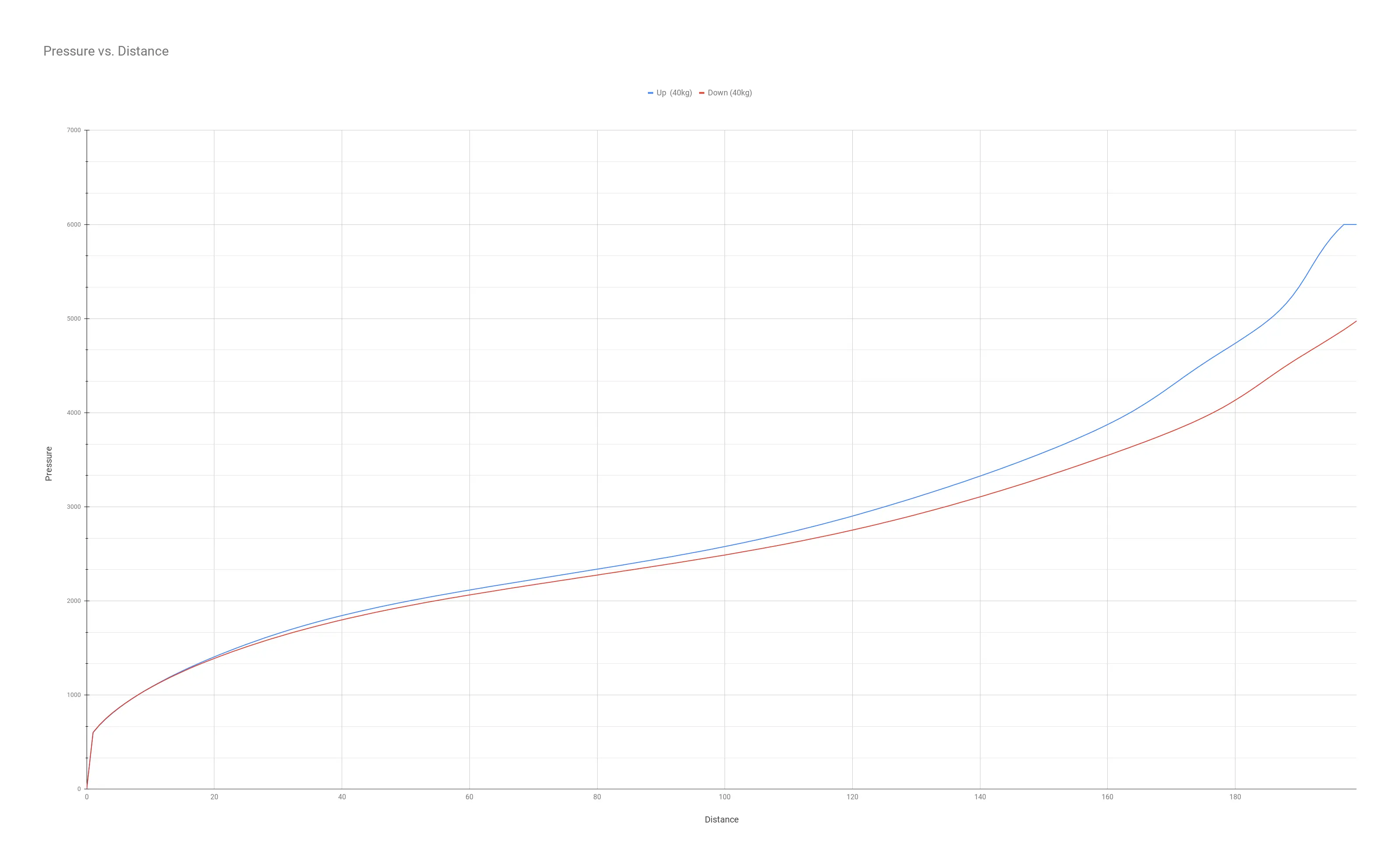
An excerpt from a bigger data set denoting distance and pressure correlation at XX kg load
| Applied pressure +ve | Distance of motion |
|---|---|
| 1217 | 14 |
| 1248 | 15 |
| … | … |
| 2488 | 100 |
| 2500 | 101 |
| … | … |
| 4176 | 182 |
| 4220 | 183 |
Missing data
Other than the above mentioned data, also required was the
- Response latency of the system when pressure is either applied or decreased
- Time taken for actuator to stabilise after application/removal of pressure or simply velocity of the actuator
Even without these timings, the work had to continue. As such I decided to research average timings for pneumatic actuators and use a sane value based on those. Making sure that the actual timings — once logged — can be substituted without any difficulty or negative consequences.
Actuator simulation methods
With the rest of the data in hand, I had multiple options of using the data.
- Storing the data in a hardcoded array — using a lookup table / map
- Using a hash table with collision detection
- Generating a curve and performing regression analysis to fit a curve to the available data, and using the function to calculate distance values for applied pressure
The lookup table and the hash table both had certain shortcomings. They both only had a single data point for each distance to pressure values, which would mean that distance value for intermediary pressure values would still have to be interpolated negating any speed gains resulting from using a lookup table/hash table.
The next issue was that even if I pre-calculate the intermediary pressure to distance values, and store it. The resulting array / dictionary would be so big — upwards of 12000 key ⇔ value pairs — that it wouldn’t be able to fit on the CPU cache. Which would mean memory I/O operations which are significantly slower. Resulting in a couple milliseconds of penalty.
The third issue was maintaining the hardcoded key ⇔ value pairs. Hard-coding is generally considered an anti-pattern. The solution to which is using external text files and/or databases. Using these external solutions would again mean expensive disk I/O operations, leading to significant time penalty. 1
The previous issue and this one only come up because our dataset, while being large enough to exceed CPU cache, is not nearly complex enough to calculate. Thus calculating the values in this case would be faster, and more I/O efficient. While still having an equal amount of time complexity.
The final issue was that the rest of the system and specifically the PID would lose granular control. The system, even though being developed on the simulation now, would eventually be used on the real platform where the pressure application can be more granular and not always a natural number.
Due to all of the above listed reasons, I decided to go with the third option, plus it gave me a chance to learn something new and it seemed more fun…
Analyzing the actuator Data
Plotting the data on a graph using matplotlib revealed a positive correlation between applied pressure and distance (Wasn’t much of a surprise, that’s how pneumatic actuators work after all).
Pneumatic muscles shrink with applied pressure, while pneumatic actuators expand. And we use pneumatic actuators, not pneumatic muscles — a point I forget later on.
Figuring out the correlation function between the two variables would help us fill in the missing data as well as provide a function that can be used inside an algorithm to determine the distance travelled upon applying pressure.
A base model was generated using a quintic function — 5th degree polynomial — for the upward motion when applying increasing pressure. And a quartic function — 4th degree polynomial — for the downward motion when applying decreasing pressure.
Regression analysis using Curve Fitting Techniques
Once the curves were generated curve fitting was performed using fityk 2 and cross-checked with SciPy 3 using the Levenberg-Marquardt algorithm
On using fityk and SciPy, I wasn’t able to get a perfect fit to the available data using the previously mentioned functions. While a perfect model seldom exists, I wanted to get as close as possible to the available data.
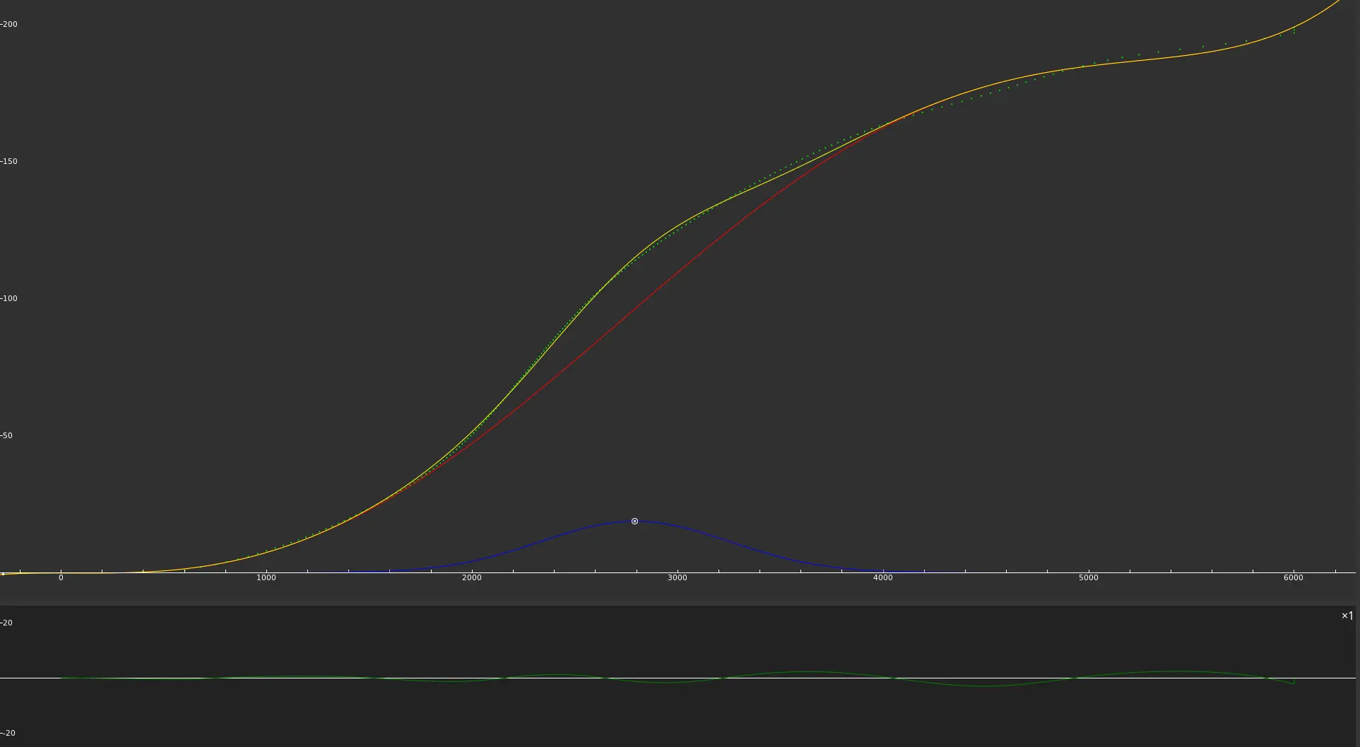
Inspection of the regression line, that is the residual vs the fitted value graph. An issue with systematic under and over-predicting the data was observed. Which is to say that the original base curve was not the best fit. Thus after trying a few different curves and still not getting the perfect fit, I moved onto creating new models for the data by combining multiple curves.
Using the regression line as a measure of the goodness-of-fit, I tried to add complements to the original quintic and quartic functions to get the residual as close to 0 as possible for every possible data point in the set of valid pressure points the system accepts. And then optimizing the fit of the new model. I finally came to a usable fit, where the residuals were random and extremely inconsequential and the r-squared was comparatively high. This model was
| Type of motion | — | Best fit function |
|---|---|---|
| Upward Motion | ⇔ | Quintic + Gaussian + Split Gaussian + Exponentially Modified Gaussian + Exponentially Modified Gaussian |
| Downward Motion | ⇔ | Quartic + Gaussian + Split Gaussian + Exponentially Modified Gaussian |
Best fit
While all of this did provide me with the best fit. Something that I should have considered earlier was whether the best fit even mattered . Because I only had access to a single set of data points for the actuator movement, and as all good statisticians are aware a single data set has a lot of inaccuracies and noise. The best solution would be to get an aggregate of multiple data sets and fit a model to the aggregated data points.
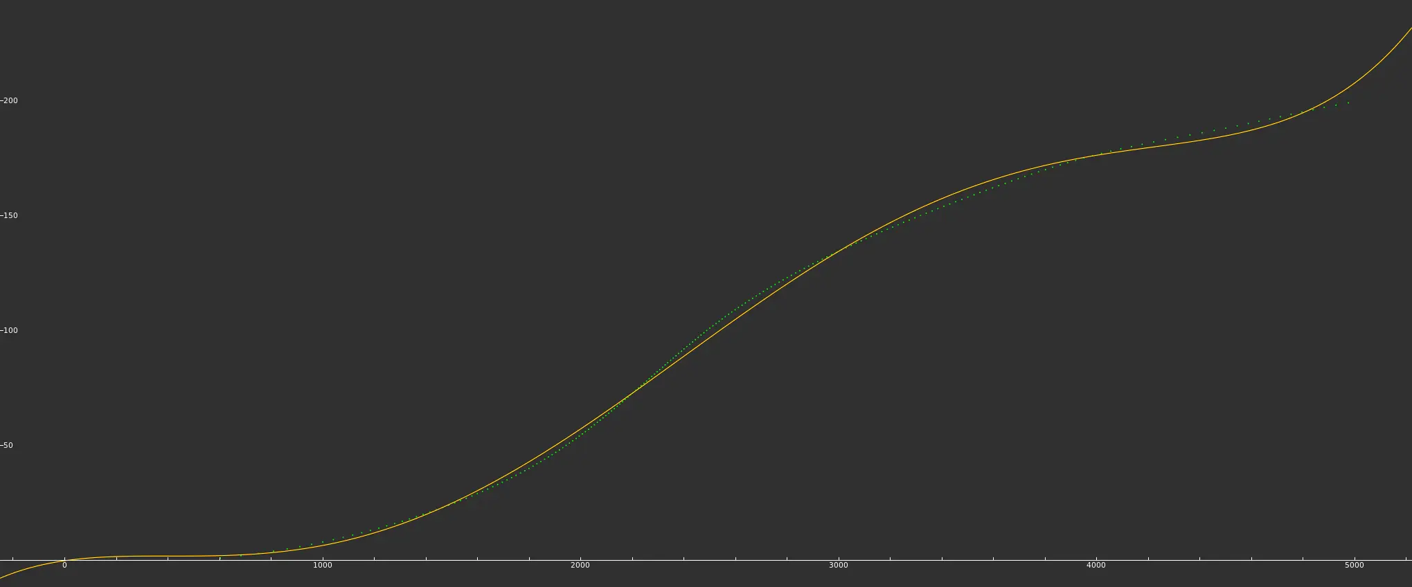
As such I decided that the complexity of the model should be reduced — dropping some of the complementary functions — to get a simple but still decently accurate mathematical model.
The model with the best fit for the requirements was
Upward Motion ⇔ Quintic + Gaussian
-0.0864580836854149382 - 0.0001004532392595508 * x - 0.0000023161937212715 * std::pow(x, 2) + 0.0000000132639645076 * std::pow(x, 3) - 0.0000000000036200247 * std::pow(x, 4) + 0.0000000000000002713 * std::pow(x, 5) + 18.8062963858669363049 * std::exp(-std::log(2) * std::pow(((x - 2792.7889820722848526202) / 540.3774049635310348094), 2))Downward Motion ⇔ Quintic
x <= 4875 ? -0.153534501375474974 + 0.016147973880630856 * x - 0.000044351093632348 * std::pow(x, 2) + 0.000000046557904348 * std::pow(x, 3) - 0.000000000012817817 * std::pow(x, 4) + 0.000000000000001097 * std::pow(x, 5) : 199Result — muscle_sim class
Yes, I mistakenly named it muscle_sim rather than actuator_sim which would have been more accurate. A simple change that I haven’t bothered to make — maybe someday…
Creates a virtual simulation of the 6 actuators on the physical platform (can also be used to simulate just a single actuator).
This class is responsible for remembering the pose of the platform, pressure in the system, some different response times of the actuators, actuator velocities, actuator motion tracking, etc. The class is considered feature complete as it implements everything required for the accurate simulation of the physical platform — bar real response times of the actuators changing response times is quite simple, and can be done once measured.
This allowed me to test the PID control system, tune the PID coefficients, gain scheduling and other components without the need for the physical system.
Test
2 test suites were created using GoogleTest along with multiple test cases and unit tests. Using sane test values, and regression testing. Providing us testing and verification of the class
2 manual tests were created with the intention to validate the generated binary and source code. Along with another manual test to validate the mathematical model against the available data


